import numpy as np
import cv2
import matplotlib.pyplot as plt

%matplotlib inline

# Load the image in a numpy array.
im = cv2.imread("./resources/elephants.jpg")
im = cv2.cvtColor(im, cv2.COLOR_BGR2GRAY)
plt.imshow(im, cmap='gray')
plt.show()
Today, we’ll explore how computers can detect patterns in images like defects or edges. We’ll start with simple kernel filters - a way to process images by looking at each pixel and its neighbors. Then, we’ll see how modern deep learning approaches automate this process, learning complex patterns from examples. Finally, we’ll examine the business case from Haiteng Engineering, where we’ll analyze whether implementing an automated quality control system makes financial sense. By the end of this session, you’ll understand the technical foundations of image analysis and how it can lead to practical business implications in manufacturing
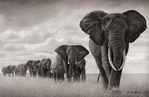
The color to black-and-white manipulation is a simple example of an image filter. By manipulating the pixels, we obtain new - sometimes unexpectedly exciting - results. Let’s load another image and create some filters for a potential new Instagram competitor ;). To keep things simple we’ll work on the black-and-white version of the image which you can download here.
import numpy as np
import cv2
import matplotlib.pyplot as plt
%matplotlib inline
# Load the image in a numpy array.
im = cv2.imread("./resources/elephants.jpg")
im = cv2.cvtColor(im, cv2.COLOR_BGR2GRAY)
plt.imshow(im, cmap='gray')
plt.show()
im.shape(392, 600)In order to be able to see the results of the amazing filters that we are going to build, we first define a function. You shouldn’t worry too much about the implementation at this point.
def plot_side_by_side(im1, im2):
    fig, axs = plt.subplots(1,2, dpi=200)
    axs[0].imshow(im1, cmap='gray')
    axs[1].imshow(im2, cmap='gray')
    plt.show()

plot_side_by_side(im, im)
Going forward, we’ll use the left part to show the original and the right part to show the transformation.
Some of the most exciting image filters are based on the principle of kernel convolution. Imagine running your fingertips over a surface to detect changes - you might feel a bump, an edge, or a smooth transition. This is exactly how kernel filters work in image processing. Just as your hand doesn’t feel just one point but rather a small area at once, these filters look at each pixel along with its neighbors. By comparing each pixel to its surrounding area in different ways (like taking averages or looking for differences), we can detect features like edges, smooth out noise, or enhance certain patterns. Depending on how we tell these ‘digital fingers’ to compare pixels with their neighbors, we can achieve different effects from smoothing out imperfections (blur) to finding sharp edges (edge detection).
A classic example is the “blur” which helps to create an air of mistery around the picture. To blur, we replace every pixel by the average of its neigbours. For instance, if we have a 3x3 image with the red focal pixel:
5 2 1
3 1 9
8 7 2
Its value would be replaced by (5+2+1+3+1+9+8+7+2)/9 = 3.66. For larger images, we would apply this to every pixel in the image. We could do this manually using for loops, but that would be … slow. Let’s be lazy and use the convolve2d function from the scipy libary instead. Not only is this a one-liner, it also runs blazingly fast!
from scipy.signal import convolve2d

weights = [
    [1/9,1/9,1/9],
    [1/9,1/9,1/9],
    [1/9,1/9,1/9]
]

im_filtered = convolve2d(im, weights, mode='same')

plot_side_by_side(im, im_filtered)
It’s hard to see, but when you focus on the grass, you see that the grass is a bit less sharp. Here’s a visualization of what the convolve2d function just did for us.
Note that the output image on the right is somewhat smaller because we have an ‘edge case’ here (edges are not included in the final result because they have no neigbours).

You try it
Increase the blur by repeatedly applying the filter.
...Ellipsisim_filtered = convolve2d(im, weights, mode='same')
im_filtered = convolve2d(im_filtered, weights, mode='same')
im_filtered = convolve2d(im_filtered, weights, mode='same')
im_filtered = convolve2d(im_filtered, weights, mode='same')
im_filtered = convolve2d(im_filtered, weights, mode='same')
im_filtered = convolve2d(im_filtered, weights, mode='same')
im_filtered = convolve2d(im_filtered, weights, mode='same')
im_filtered = convolve2d(im_filtered, weights, mode='same')
plot_side_by_side(im, im_filtered)
You can increase the effect by taking a larger neighborhood of, say, 4 pixels above/below (8*8 in total). Let’s also use the np.ones(size) function instead of typing out the large matrix.
weights     = np.ones((8,8)) / 64
im_filtered = convolve2d(im, weights, mode='same')
plot_side_by_side(im, im_filtered)
Often, we will want to be able to detect things in images: number of people, faces of people, defects in a product, etc. A first step to object detection is to apply edge detection.
A simply trick we can use is to use a kernel, but just take into consideration anything on the left and the right. This way, you will detect strong changes in the horizontal direction:
        -1 0 1
        -2 0 2
        -1 0 1
To use the hand analogy: just as your fingertips can feel a sudden change in height when running across the edge of a table, this filter detects sudden changes in brightness between neighboring pixels. The negative numbers on the left and positive numbers on the right act like fingertips detecting the ‘step up’ or ‘step down’ in pixel values from left to right.
Try programming applying the above filter to the image.
from scipy.signal import convolve2d

weight_edge_hor = [
    [-1,0,1],
    [-2,0,2],
    [-1,0,1]
]

im_edge_hor = convolve2d(im, weight_edge_hor, mode='same')
plot_side_by_side(im,im_edge_hor);
White means that the it’s detecting an edge from left to right, black means that it’s detecting an edge from right to left. Grey means nothing was detected.
We can achieve a similar effect for the horizontal direction:
from scipy.signal import convolve2d
weight_edge_ver = [
    [-1,-2,-1],
    [ 0, 0, 0],
    [ 1, 2, 1]
]

# alternatively:
weight_edge_ver = np.array(weight_edge_hor).T

im_edge_ver = convolve2d(im, weight_edge_ver, mode='same')
plot_side_by_side(im,im_edge_ver);
If we want to detect all edges, we can apply the Sobel formula which we program here without worrying about the mathematical detail.
im_edge = np.sqrt(im_edge_hor**2 + im_edge_ver**2)

plot_side_by_side(im,im_edge);
As a final exercises for today, try applying your favourite filter from above using the code below. Before you run the code, pay attention to the following:
# Your filter implementation goes here.
def my_filter(im):

    #nofilter ;)

    # define your filter here!
    # ...
    # end of your filter

    return im
### Boilerplate code to get the filter running, don't change me
# First, we get the camera device from your computer
cv2.startWindowThread()
camera = cv2.VideoCapture(0)
try:
while True:
# Capture frame-by-frame
ret, im = camera.read()
if not ret:
print("Failed to grab frame")
break
# Convert to grayscale
im = cv2.cvtColor(im, cv2.COLOR_BGR2GRAY)
# Resize for performance if you're working on a slow computer
resize_factor = 1
im = cv2.resize(im, (int(im.shape[1]/resize_factor),
int(im.shape[0]/resize_factor)))
# Apply filter
im = my_filter(im)
# Display the result
cv2.imshow('Pynstagram v1.0', im.astype(np.uint8))
# Break loop with 'q' key
if cv2.waitKey(1) & 0xFF == ord('q'):
break
finally:
# Clean up, release camera etc.
camera.release()
cv2.destroyAllWindows()
for i in range(4):
cv2.waitKey(1)Here’s an interesting one:
weight_edge_hor = [
    [-1,0,1],
    [-2,0,2],
    [-1,0,1]
]
weight_edge_ver = [
    [-1,-2,-1],
    [ 0, 0, 0],
    [ 1, 2, 1]
]

# Your filter implementation goes here.
def my_filter(im):
    # Dreamy brightness
    #im = im.astype(np.uint32) * 2
    #im = np.clip(im,0,255)

    # Blur
    #weights = np.ones((8,8))/64
    #im = convolve2d(im, weights, mode='same')

    # Edge detection
    im_edge_ver = convolve2d(im, weight_edge_hor, mode='same')
    im_edge_hor = convolve2d(im, weight_edge_ver, mode='same')
    im = np.sqrt(im_edge_hor**2 + im_edge_ver**2)


return imWhat we have learned so far is the basis of computer vision, which we’ll talk more about in the next class. To get a feeling, try out the following example which does face detection. It requires that you download a predefined filter (it’s quite large matrix of numbers!) which you can download from here.
Note, this filter is called a Haar filter, which is like the edge detection that we did, but with some extra mathematical bells and whistles to it. This is one, specifically, is coupled with routines to be able to detect the position of a face in an image.
import numpy as np
import cv2

def my_filter(im):
    # Load the cascade
    face_cascade = cv2.CascadeClassifier('./resources/haarcascade_frontalface_default.xml')

    # Detect faces - assumes grayscale
    faces = face_cascade.detectMultiScale(im, 1.1, 4)

    # Draw rectangle around the faces
    for (x, y, w, h) in faces:
        cv2.rectangle(im, (x, y), (x+w, y+h), (255, 0, 0), 2)

    return im

### Boilerplate code to get the filter running, don't change me
# First, we get the camera device from your computer
camera = cv2.VideoCapture(0)
cv2.startWindowThread()

while(True):
    # Capture frame-by-frame the R,G,B values of the camera
    ret, im = camera.read()

    # We work on grayscale by default, but you can uncomment
    # this line to get the full color spectrum.
    im = cv2.cvtColor(im, cv2.COLOR_BGR2RGB)

    # Here, we resized the image to ensure that the your computer
    # can handle the calculations in real-time. You may have to set
    # the resize factor to 2, or even 4 on your computer depending
    # on how fast your computer is.
    resize_factor = 1
    im = cv2.resize(im, (int(im.shape[1]/resize_factor), int(im.shape[0]/resize_factor)))

    # Now, we apply the filter that you created to the image
    im = my_filter(im)

    im = cv2.cvtColor(im, cv2.COLOR_RGB2BGR)

    cv2.imshow('Face Detection v1.0', im.astype(np.uint8))
    if cv2.waitKey(1) & 0xFF == ord('q'):
        break

camera.release()
cv2.destroyAllWindows()
cv2.waitKey(1);We’ve seen how kernel filters can detect edges and patterns in images. Modern quality control systems take this idea further using Convolutional Neural Networks (CNNs). Think of a CNN as an automated system that:
A classic version of a CNN could look as follows:

While this may look complex at first, note that the actual procedure to apply this is quite similar to what we’ve done so far.
The implementation follows four key steps:
Step1: Set-up the System
I have already trained a neural network to do the detection for you, download it along with the other resources here an place it in a folder that is accessible to python. You can load the pre-trained model that has already learned to detect defects from thousands of examples.
RESOURCE_FOLDER = './resources/haiteng'import cv2
import numpy as np
import os
from pathlib import Path
# Define possible outcomes
classes = ['OK', 'defect']
# Load our pre-trained model
net = cv2.dnn.readNetFromONNX(RESOURCE_FOLDER + "/cast_classifier.onnx"))
# Function to load our dataset
def load_image_dataset(dataset_file):
data = np.genfromtxt(dataset_file, delimiter=',', dtype=str)
file_names = data[:, 0] # First column: image names
labels = data[:, 1] # Second column: true labels (0=OK, 1=defect)
return file_names[1:], labels[1:].astype(int) # Skip header rowStep 2: Analyze Images
The model processes each image through multiple layers of filters, let’s define the function to do so and try it out on a single image.
def classify_image(filename):
    try:
        # Load and preprocess the image
        image = cv2.imread(filename)
        blob  = cv2.dnn.blobFromImage(image,
                                    scalefactor=1/255.0,
                                    size=(224, 224),
                                    swapRB=True)

        # Get model's prediction
        net.setInput(blob)
        logits = net.forward()

        # Convert to probabilities
        exp_logits = np.exp(logits - np.max(logits, axis=1, keepdims=True))
        probabilities = exp_logits / np.sum(exp_logits, axis=1, keepdims=True)
        return probabilities

    except cv2.error as e:
        print("Couldn't load the file, are you sure the path is correct?")
        return

# Let's run it on one image, change the image name on the right if you want
# to try it on other ones.
test_image = str(Path(RESOURCE_FOLDER) / "images" / "def_front_cast_def_0_7.jpeg")

result = classify_image(test_image)

if(result is not None):
    print(f"Probabilities for {test_image}:")
    print(f"OK:               {result[0,0]:.1%}")
    print(f"Defect:           {result[0,1]:.1%}")
Probabilities for resources/haiteng/images/def_front_cast_def_0_7.jpeg:
OK: 9.9%
Defect: 90.1%Step 3 and 4 are part of your first take-home challenge!